Data Sources - Freshwater Health Index

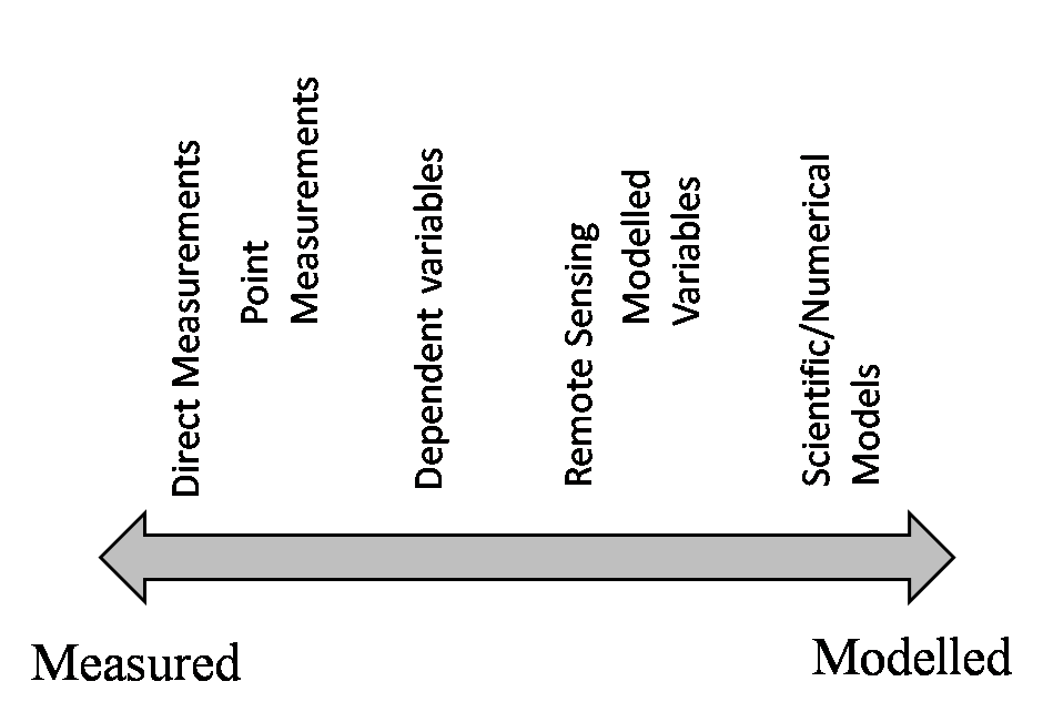
Data required to calculate the indicators at the sub-basin and basin level is expected to come from a variety of sources combining in-situ measurements, remotely-sensed information and modelled outputs (Figure 4). While direct or in-situ measurement can claim to have the advantage of being the “real” value of variable being measured, such data is both labor intensive to collect and spatially sparse. Remotely-sensed information, on the other hand, may have poorer point accuracy, but have larger and more consistent spatial coverage and ability to identify spatial and temporal patterns. Data from numerical models helps fill in the gaps on ‘measured’ data availability and provide information on inferred or derived variables, but are dependent on the quality of inputs and the characterization of the complex processes they are attempting to simulate.

Figure 4. Data sources and types. The graph ranges from direct empirical data that is collected on the ground to scientific and numerical models which use direct measurements or variables derived from remote sensing. Direct measurements are data usually in the form of point estimates; however, when numerous such points are collected through space and time (or with respect to some other variable), they can be used to create a distribution. Dependent variables are simple mathematical or statistical functions of direct measurements. Remote sensing data typically needs to be converted via more complex functions or statistical methods into a useful metric. Scientific/numerical models refers to complex models that might use any of the above forms of input.

Each basin is expected to have its own suite of data monitoring sources and models based on a number of local, regional and global factors – such as capability of local authorities, institutional importance for certain physical variables (e.g., water quality), scale of the basin being studied, etc. Table 6 tabulates some examples of local or remotely-sensed data, alongside hydrological, groundwater, hydraulic, water quality, and ecosystem service models (among others) that may be relevant to, or used by, institutions in the basin. Adopting the guidelines documented in Sections 5 and 6 should inform the user of the underlying data required and permit the calculation of the indicators.

Table 6. Local and global data sources, models and metrics for evaluating Ecosystem Vitality and Ecosystem Services indicators

Major indicator	Sub-indicator	Metrics/models	Local and site-scale datasets and models	Global and regional datasets and models
Ecosystem Vitality
Water Quantity	Deviation from Natural Flow Regime	AAPFD (Gehrke et al., 1995), Hydrologic Deviation (Ladson et al., 1999)	River gauges, hydrological models such as SWAT, HSPF, GSFLOW, etc.	Calibrated instance of Global Hydrologic Models/Land Surface Models such as VIC, WaterGAP, etc.
	Groundwater Storage Depletion	% Area affected	Monitoring wells	GRACE satellite data, land subsidence studies using SAR
Water Quality	Water Quality Index (from TSS, TN, TP and others)	Aggregate of parameter missing WQ targets with frequency and amount with which targets are not met	Local monitoring station, Water quality models such as QUAL, WASP, etc.	MODIS and VIIRS water quality parameters
Drainage Basin Condition	Bank Modification	Percent of bank/shoreline modified	Aerial Photography	LandSAT imagery, SAR (like Sentinel 1) imagery
	Flow connectivity	Dendritic Connectivity Index (Cote et al. 2009)	Aerial Photography; government database on dam and weir locations	GRanD (Global Reservoir and Dam) Database
	Land cover naturalness	Naturalness Index based on land cover, 0-100 scale	Aerial Photography, Local survey for land use	MODIS land cover, Global Forest Change database, ESA CCI land cover products
Biodiversity	Change in richness and	% Change in number of species and abundance	Local survey	IUCN Red List, national and regional threatened species lists, Global Population Dynamics Database; Global Invasive Species Database
	population size of species of concern
	Change in richness and population size	% Change in number of species and abundance
	of invasive and nuisance species
Ecosystem Services
Provisioning	Water supply reliability relative to demand	Aggregate of sites affected,	Government regulation records, Water supply and demand models such as WEAP	Water availability information from Global Hydrologic Models/Land Surface Models. Demand estimates based on changes in soil moisture, evapotranspiration, etc. (Nazemi and Wheater, 2015)
		frequency and amplitude of gap between water supply and demand
	Biomass for consumption	Amount of production or area contributing to biomass, frequency and amplitude of gap between biomass supply and demand	Local monitoring data	N/A
Regulation and Support	Sediment regulation	Aggregate of areas affected, frequency and amount of changes in sediment deposition and erosion thresholds	Reservoir operation and regulation records, hydrological models, Ecosystem service models such as InVEST, ARIES	LandSAT or other high resolution imagery, SAR surveys
	Water quality regulation	Aggregate of parameter missing WQ targets with frequency and amount with which targets are not met	Local monitoring stations and authorities	MODIS and VIIRS water quality parameters
	Flood regulation	Aggregate of sites affected, frequency and amplitude of floods compared to demand	Hydrological models and hydraulic models such as HEC-RAS,etc	NRT Global flood mapping, Global flood risk models (Ward et al, 2015)
	Disease regulation	Aggregate of areas affected, incidence ratio and case-to-fatality ratio	Local monitoring and authorities; WADI modelling approach	Resources such as complied by WHO, Global Infectious Disease and Epidemiology Network (GIDEON), generalized global models from Yang et al (2012)
Cultural	Conservation/Cultural Heritage sites	Area (can be weighted by perceived value)	Government regulation records	World Database on Protected Areas
	Recreation	Person-use days or travel costs	Local survey	Geotagged photographs from social media sites

Setting up a Basin Study Data Sources